Stanford cs231n: Optimization Algorithms in Neural Networks
In this post, Optimization Algorithms in Neural Network will be explained. Thanks to Stanford University, the lecture videos of cs231n can be found in YouTube and all materials are freely available (see the references).
First Order Optimization Algorithms
- SGD
- SGD with Momentum
- SGD with Nesterov Momentum
- AdaGrad
- RMSProp
- Adam
SGD
w = w - learningrate * gradient
- Vanilla update.
- The simplest form of update is to change the parameters along the negative gradient direction
- Since the gradient indicates the direction of increase, but we usually wish to minimize a loss function
SGD with Momentum
velocity = 0
velocity = momentum * velocity - learningrate * gradient
w = w + velocity
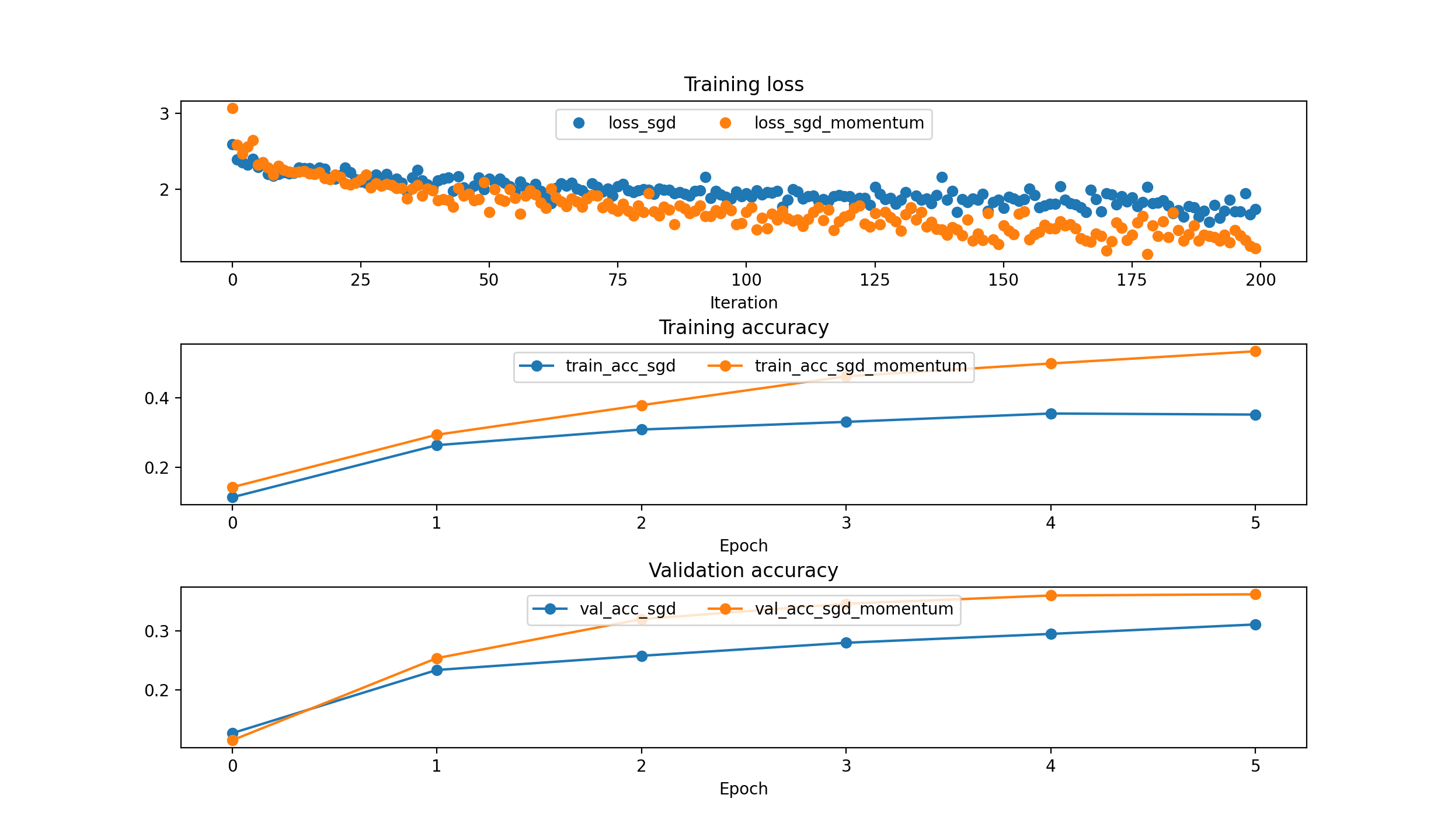
- With Momentum update, the parameter vector will build up velocity in any direction that has consistent gradient.
SGD with Nesterov Momentum
old_velocity = velocity
velocity = momentum * velocity - learningrate * gradient
w = w + (-momentum) * old_velocity + (1- (-momentum)) * velocity
- https://arxiv.org/pdf/1212.0901v2.pdf : ADVANCES IN OPTIMIZING RECURRENT NETWORKS
- http://www.cs.utoronto.ca/~ilya/pubs/ilya_sutskever_phd_thesis.pdf : RNN
AdaGrad
Ref: https://jmlr.org/papers/volume12/duchi11a/duchi11a.pdf (-) Ref: https://arxiv.org/pdf/1212.5701.pdf *
gradient_squared = 0
gradient_squared += gradient**2
w += - learning_rate * gradient / (np.sqrt(gradient_squared) + eps)
Pros: *
While there is the hand tuned global learning rate, each dimension has its own dynamic rate.
Since this dynamic rate grows with the inverse of the gradient magnitudes: - large gradients have smaller learning rates - small gradients have large learning rates.
This is very beneficial for training deep neural networks since the scale of the gradients in each layer is often different by several orders of magnitude, so the optimal learning rate should take that into account.
Accumulation of gradient in the denominator has the same effects as annealing, reducing the learning rate over time.
Cons: *
- This method can be sensitive to initial conditions of the parameters and the corresponding gradients.
- If the initial gradients are large, the learning rates will be low for the remainder of training.
- This can be combatted by increasing the global learning rate, making the ADAGRAD method sensitive to the choice of learning rate.
- Due to the continual accumulation of squared gradients in the denominator, the learning rate will continue to decrease throughout training, eventually decreasing to zero and stopping training completely.
- Another exp: A downside of Adagrad is that in case of Deep Learning, the monotonic learning rate usually proves too aggressive and stops learning too early. **
RMS Prop
gradient_squared = 0
gradient_squared = decay_rate * gradient_squared + (1 - decay_rate) * gradient**2
w += - learning_rate * gradient / (np.sqrt(gradient_squared) + eps)
- The RMSProp update adjusts the Adagrad method in a very simple way in an attempt to reduce its aggressive, monotonically decreasing learning rate.
- In particular, it uses a moving average of squared gradients.
-
decay_rate is a hyperparameter and typical values are [0.9, 0.99, 0.999].
- Notice that the w+= update is identical to Adagrad.
- But the gradient_squared variable is a “leaky”. (has decay rate)
- Hence, RMSProp still modulates the learning rate of each weight based on the magnitudes of its gradients. It has a beneficial equalizing effect.
- But unlike Adagrad, the updates do not get monotonically smaller.
Adam
Ref: https://arxiv.org/pdf/1412.6980.pdf
# t is your iteration counter going from 1 to infinity
first_moment, second_moment = 0, 0
for t in range(iterations):
    first_moment = beta1 * first_moment + (1-beta1) * gradient
    first_unbias = first_moment / (1-beta1**t)

    second_moment = beta2 * second_moment + (1-beta2)*(gradient**2)
    second_unbias = second_moment / (1-beta2**t)

    w += - learning_rate * first_unbias / (np.sqrt(second_unbias) + eps)
The method computes individual adaptive learning rates for different parameters from estimates of first and second moments of the gradients; the name Adam is derived from adaptive moment estimation.
Without bias:
At very first time step, second moment is zero. After one update teh second moment will still close to zero. When we divide by second moment, we make a very large step at the beginning. But this big step is not related with the geometry of the loss function, it is the nature of the formula.
Bias correction term help to aviod the very large step at the beginning.
You can start with these parameters:
beta1 = 0.9
beta2 = 0.999
lr = 1e-3 or 1e-5
RMSProp with momentum generates its parameter updates using a momentum on the rescaled gradient, whereas Adam updates are directly estimated using a running average of first and second moment of the gradient.
RMSProp also lacks a bias-correction term; this matters most in case of a value of beta2 close to 1 (required in case of sparse gradients), since in that case not correcting the bias leads to very large stepsizes and often divergence.
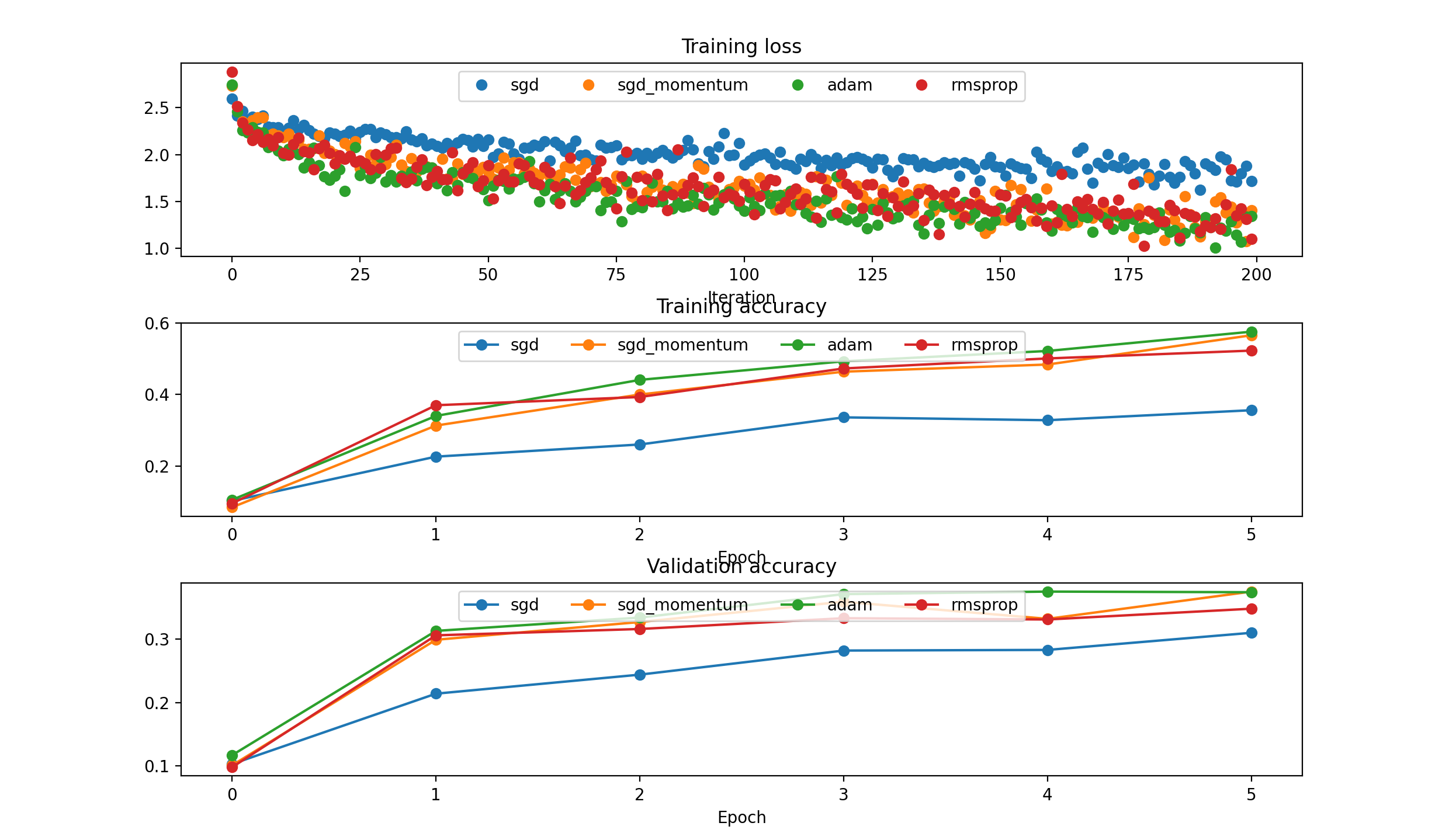
Different Models comparison: {‘sgd’: 5e-3, ‘sgd_momentum’: 5e-3, ‘rmsprop’: 1e-4, ‘adam’: 1e-3}
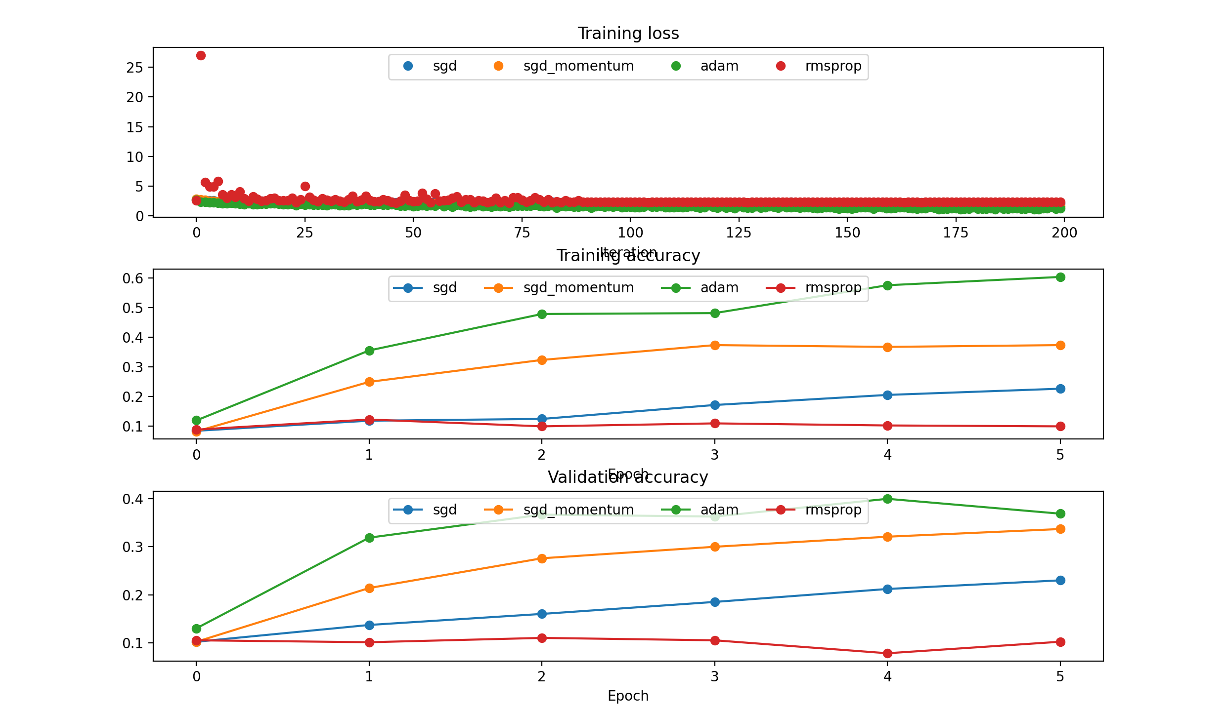
Different Models comparison: {‘sgd’: 1e-3, ‘sgd_momentum’: 1e-3, ‘rmsprop’: 1e-3, ‘adam’: 1e-3}
Change LR
you can change learning rate during the training:
- Step Decay
- Exponential Decay
- 1/t decay
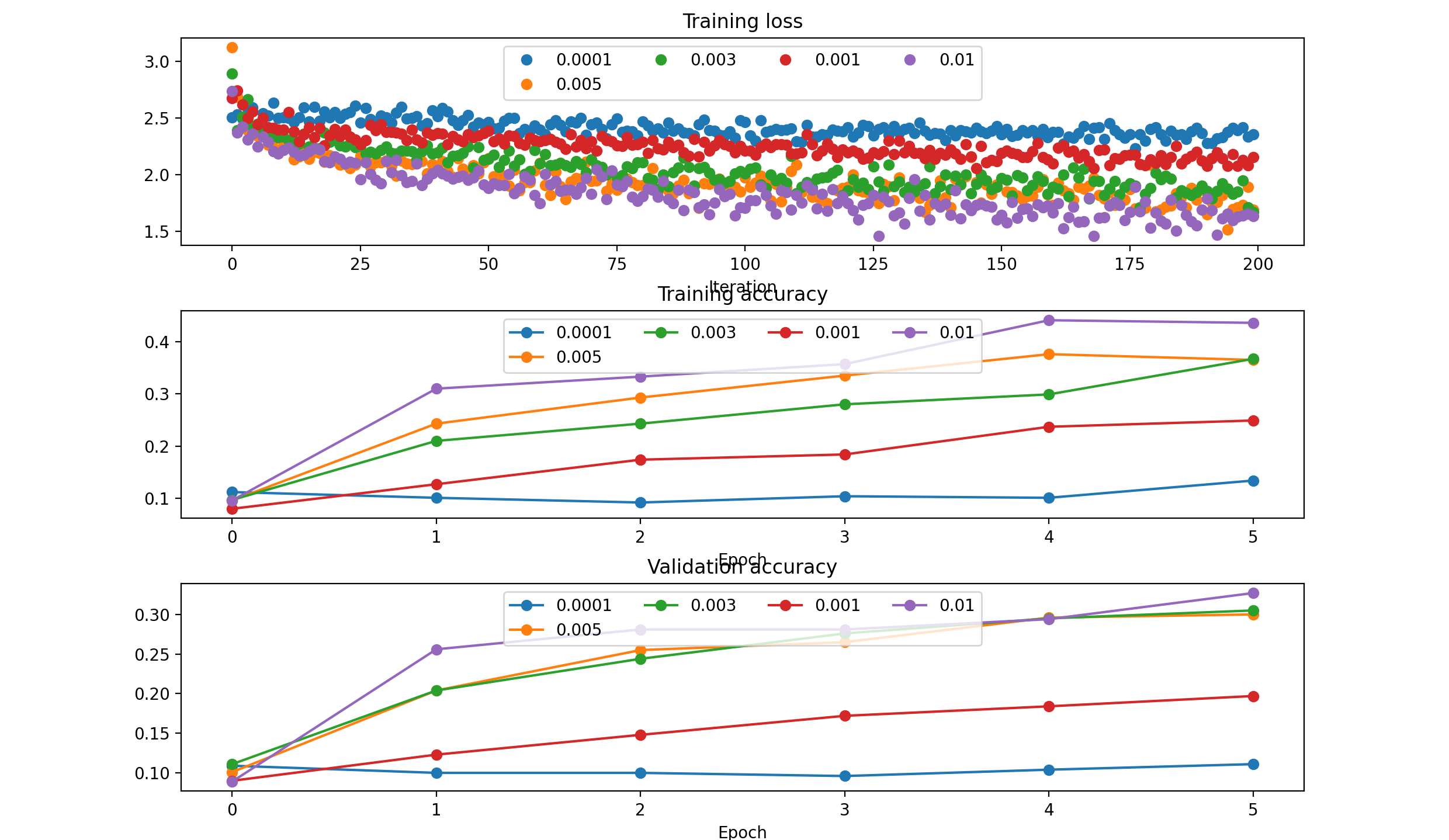
Start with no decay. Select the best learning rate. Check the loss plot and decide where you need decay.
‘sgd’ :
‘sgd_momentum’:
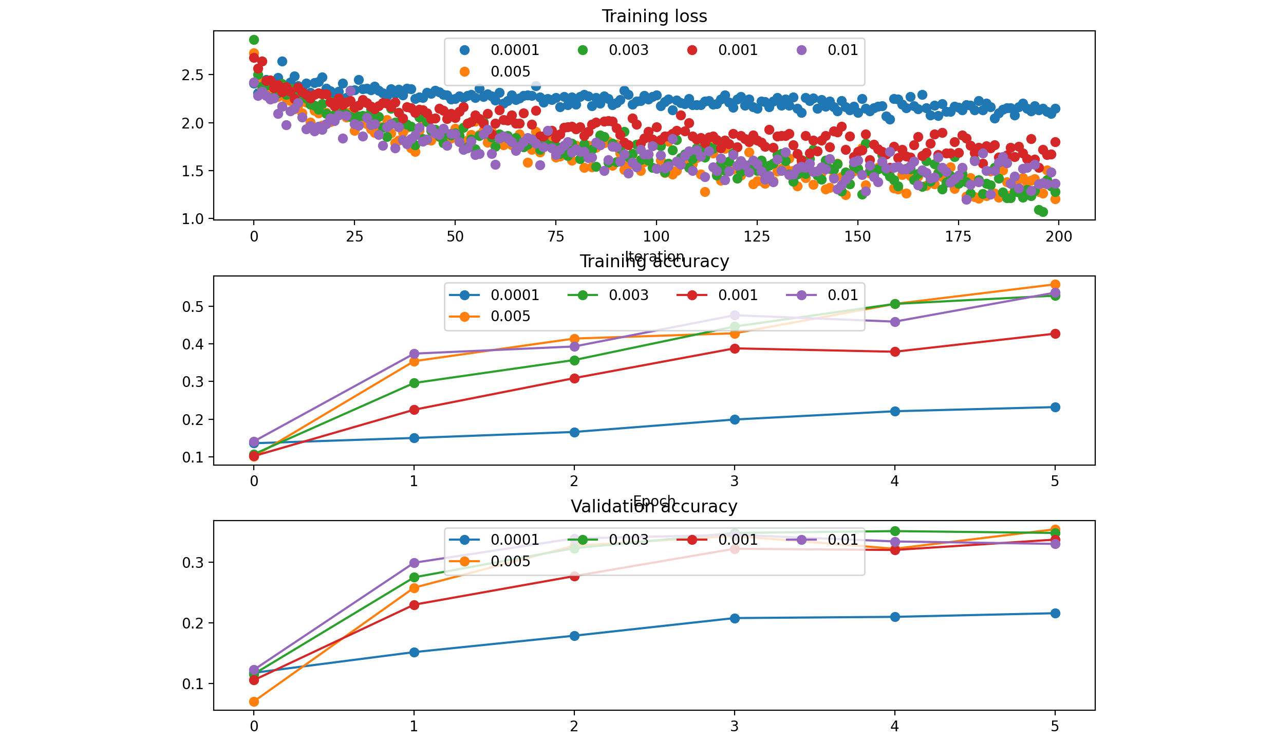
‘rmsprop’:
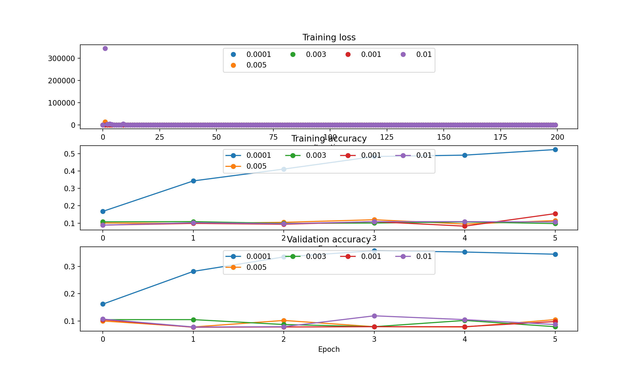
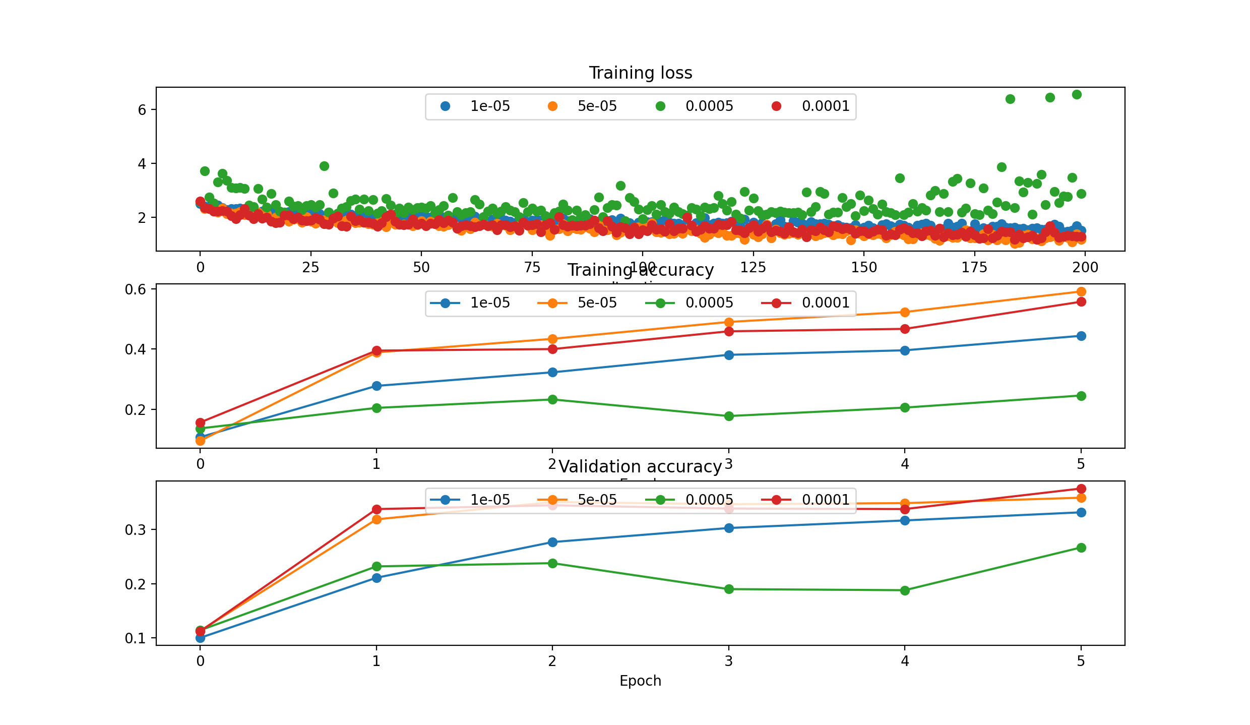
RMS Prop needs smaller lr: [1e-5, 5e-5, 5e-4, 1e-4]
- running with 5e-05: (Epoch 5 / 5) train acc: 0.591000; val_acc: 0.359000
- running with 0.0001: (Epoch 5 / 5) train acc: 0.557000; val_acc: 0.376000
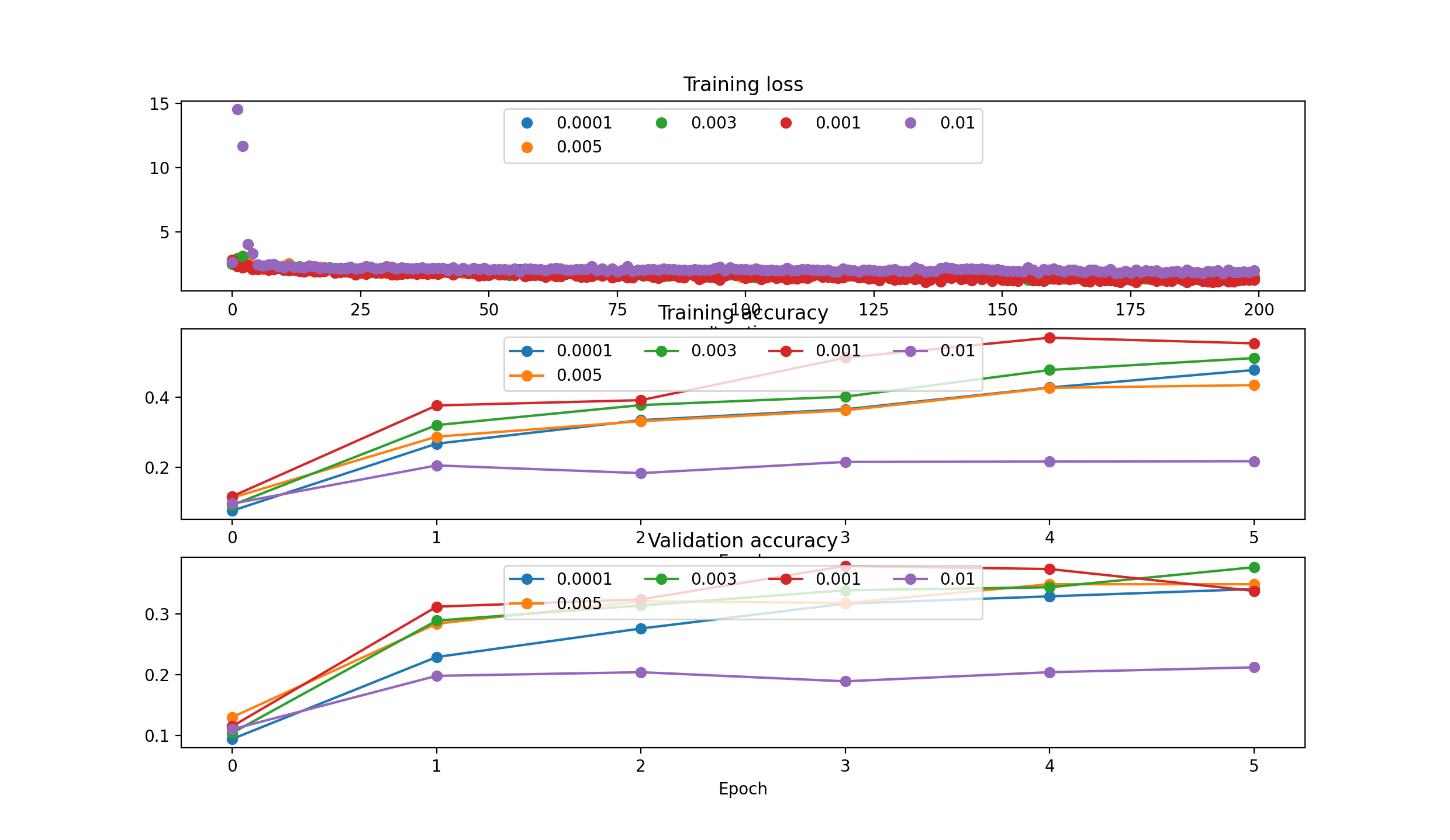
####’adam’:
Model Ensembles
Ref: https://www.youtube.com/watch?v=EK61htlw8hY&ab_channel=TTIC
One disadvantage of model ensembles is that they take longer to evaluate on test example. An interested reader may find the recent work from Geoff Hinton on “Dark Knowledge” inspiring, where the idea is to “distill” a good ensemble back to a single model by incorporating the ensemble log likelihoods into a modified objective.
Ref: https://www.youtube.com/watch?v=_JB0AO7QxSA&list=PL3FW7Lu3i5JvHM8ljYj-zLfQRF3EO8sYv&index=7&ab_channel=StanfordUniversitySchoolofEngineering
- Train multiple independent models
- At test time average their results
Second Order Optimization Algorithms
- https://arxiv.org/pdf/1311.2115.pdf (Quasi Newton)
- https://research.google/pubs/pub40565/ (Large Scale Distributed Deep Networks)
- https://en.wikipedia.org/wiki/Limited-memory_BFGS (LBFGS)
References
- https://www.youtube.com/watch?v=_JB0AO7QxSA&list=PL3FW7Lu3i5JvHM8ljYj-zLfQRF3EO8sYv&index=7&ab_channel=StanfordUniversitySchoolofEngineering
- https://cs231n.github.io/
Key Words
SGD, Momentum, Learning Rates, RMSProp, ADam, Optimization, Neural Networks